VINDTA DIC processing

koolstof only deals with dissolved inorganic carbon (DIC) measurements. For total alkalinity, use Calkulate.

koolstof provides a set of functions to import VINDTA data files as pandas DataFrames and then perform in-place operations on them to process and calibrate the data, plus some plotting functions. There are two main processing steps: (1) applying the blank correction, and (2) calibrating to CRMs.

Breaking changes in v0.25

The way in which VINDTA processing works has been significantly overhauled as of koolstof v0.25. In particular, the Dbs class no longer exists, so the functions described here can no longer be called as methods from the imported dbs file. In general, the change will look something like this:

dbs.do_something()     # old version, pre-v0.25
ksv.do_something(dbs)  # new version, v0.25 onwards

But some functions have been completely renamed and their inputs/outputs changed. Update with caution and read the new instructions below carefully!

All the examples here assume the following import convention:

from koolstof import vindta as ksv

Import VINDTA files

The logfile.bak

Import a logfile.bak into a standard pandas DataFrame with one row per DIC sample.

logfile = ksv.read_logfile("path/to/logfile.bak", methods="3C standard")

read_logfile: optional keyword arguments

• methods: list of VINDTA method filenames used to run samples, excluding the .mth extensions

The dbs file

Import a .dbs file into an enhanced DataFrame and rename its columns into a friendlier format.

dbs = ksv.read_dbs("path/to/file.dbs", keep_all_cols=False)

read_dbs: optional keyword arguments

• keep_all_cols: retain all columns from the .dbs (True) or just the most important ones (False)?

Add sample metadata

Once you've imported the files above, you need to add the following metadata as extra columns in the dbs DataFrame under the following column labels:

• "salinity": practical salinity (assumed 35 if not provided)
• "temperature_analysis_dic": temperature of DIC analysis in °C (assumed 25 °C if not provided)
• "dic_certified": certified DIC values for reference materials in μmol/kg-sw. Non-reference samples should be set to np.nan.

You can also add the following logical columns to refine which samples and reference materials are used for processing and calibration:

• "blank_good": use this sample in assessing the coulometer blank value?
• "k_dic_good": use this reference material for calibration?

As a starting point, you could set all "blank_good" values to True and "k_dic_good" to True for all CRMs but False everywhere else.

A complete example script up to this point might look something like this:

import numpy as np
from koolstof import vindta as ksv

# Import files from VINDTA
logfile = ksv.read_logfile("path/to/logfile.bak")
dbs = ksv.read_dbs("path/to/dbsfile.dbs")

# Assign certified DIC for CRMs
# - In this example, we assume that the 'bottle' column of the dbs always
#   starts with the letters "CRM" for CRMs, and that all CRMs have a
#   certified value of 2017.45 µmol/kg
dbs["dic_certified"] = np.where(
    dbs.bottle.str.startswith("CRM"), 2017.45, np.nan
)

# Assign analysis temperature, if it's not 25 °C
dbs["temperature_analysis_dic"] = 23.0

# Assign dbs["salinity"] here too, if it's not always 35

# Set up logicals
dbs["blank_good"] = True
dbs["k_dic_good"] = ~dbs.dic_certified.isnull()

Now we're ready to apply the blank corrections and then calibrate.

Find and apply blank corrections

To find and apply the blank corrections, use ksv.blank_correction().

sessions = ksv.blank_correction(
    dbs,
    logfile,
    blank_col="blank",
    counts_col="counts",
    runtime_col="run_time",
    session_col="dic_cell_id",
    use_from=6,
)

blank_correction: optional keyword arguments

• blank_col: the name of the column containing the blank for each sample.
• counts_col: the name of the column containing the raw counts for each sample.
• runtime_col: the name of the column containing the total run time for each sample.
• session_col: the name of the column containing the analysis session identifiers.
• use_from: which minute of the coulometric titrations to measure the blank starting from.

The output sessions is a table of analysis sessions, as identified by unique values of the session_col. The dbs is also updated with extra columns, most importantly, "blank_here" and "counts_corrected".

After running blank_correction, you should make a few plots to check that everything has worked as intended.

Plot the count increments

First, check that you are using an appropriate value of use_from. In general, in a coulometric titration, all the CO₂ from the sample passes through the coulometer within the first few minutes, so the last few minutes can be considered as 'blank' measurements. koolstof determines the blank first on a sample-by-sample basis starting from whatever minute is specified by use_from, so we should check that the increments from this point actually are constant. To do this:

ksv.plot_increments(dbs, logfile, use_from=6)

This generates a figure like below:

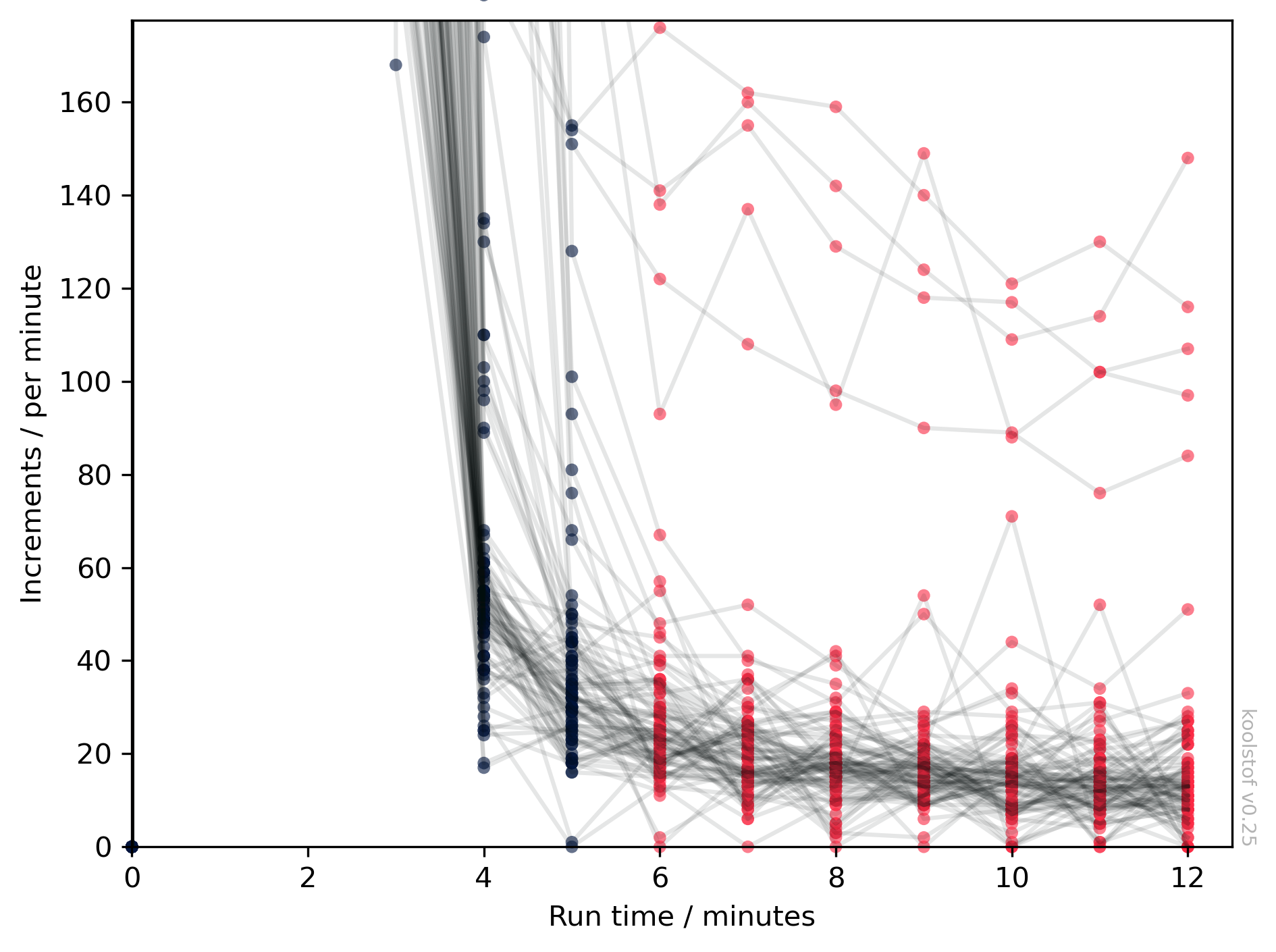
Here we see the count increments for every sample in the dbs. The y-axis is automatically zoomed in on the lower values at the end of the analysis, which we use to determine the blank. The data points currently considered as 'blanks', where the number of minutes is greater than or equal to use_from, are shown in red. We need to check that all the sample has indeed passed through this point, and that there isn't a strong trend with time in the red points.

In the example above, the points at minute 6 (and possibly 7) are still a bit higher than the points later on, so it would probably be better to switch to use_from=7 (or use_from=8) when running ksv.blank_correction on this dataset.

Plot the session blank fits

Once we're happy with the use_from value, we can plot the blank fits on a session-by-session basis. Although we determine an individual blank value for each sample, koolstof doesn't use these directly to make the blank correction. The results are better if you fit a curve through the blank values for each analysis session. To visualise the fitted curves for all the analysis sessions in your dbs, use:

ksv.plot_blanks(dbs, sessions)

This generates a sequence of plots, each something like this:

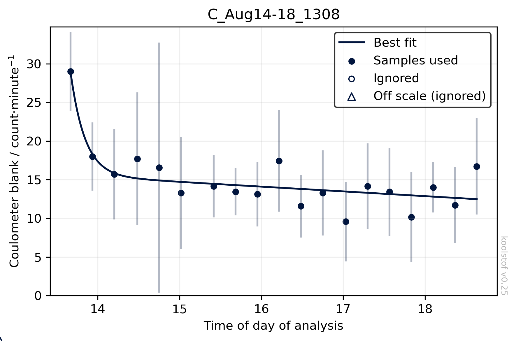
The points are the sample-by-sample blank values, with error bars indicating the standard deviation of the minute-by-minute blank estimates for each sample. The solid line shows the fit, which is what's actually used to make the blank correction for each sample.

If any points fall far away from the rest and are causing the solid line to not have a good fit to the data, you can ignore them (in this curve fitting step only) by setting the "blank_good" column of dbs to False for those rows. Then, re-run ksv.blank_correction. These points will subsequently show up as open symbols on these plots (see legend - 'Ignored') and won't influence the fitted line.

A DIC result will still be returned for these points, so you should check whether it looks sensible, as an unusual blank value may indicate that something may have gone wrong with that particular analysis.

Calibrate DIC measurements

Once the blank correction is complete, you can calibrate the DIC measurements based on CRMs.

ksv.calibrate_dic(dbs, sessions)

This adds extra columns to dbs and sessions with various calibration metadata. The final DIC result can be found in dbs.dic.

Next, you should visualise the calibration factors and exclude any bad CRM measurements from the calibration.

Plot calibration factors

To see all the calibration factors in the dbs through time, use:

ksv.plot_k_dic(dbs, sessions, show_ignored=True)

The plot may look something like this:

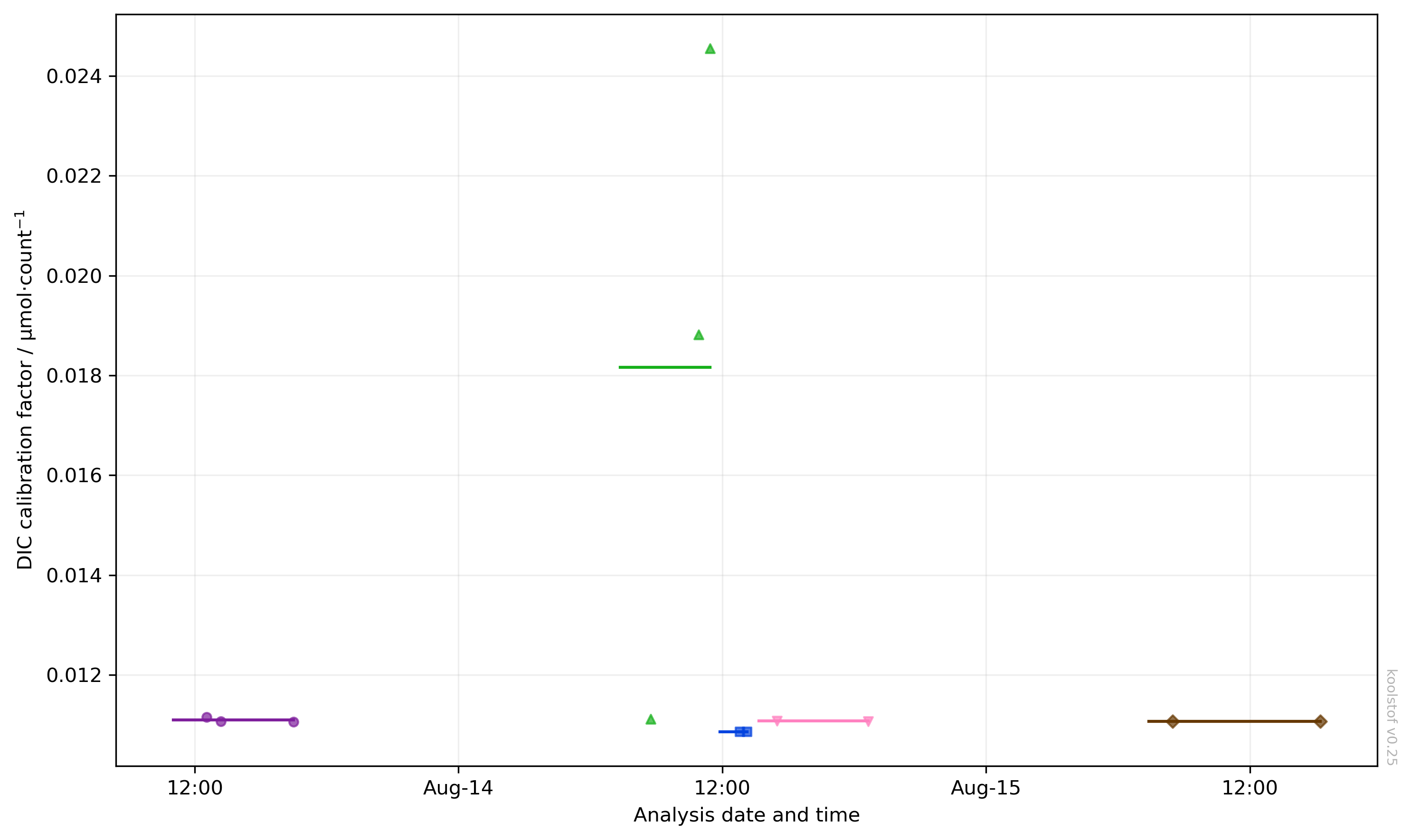
Each change of colour and marker style indicates a new analysis session, and the horizontal lines show the mean calibration factors used for each session.

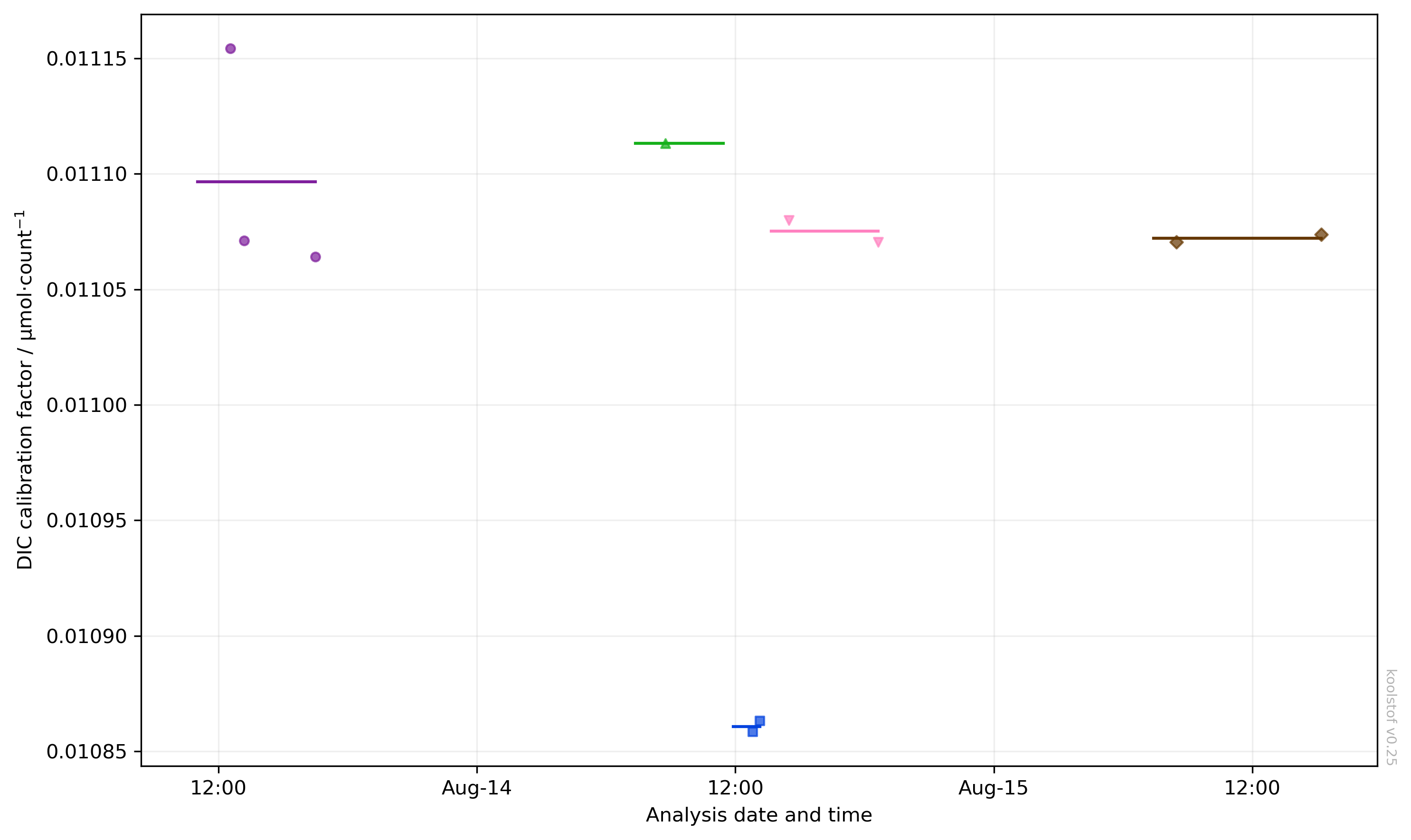
In the example above, there are clearly two bad CRM measurements. You can exclude these from the calibration by setting "k_dic_good" to false, then re-run ksv.calibrate_dic to recalibrate. Recreating the figure above but with show_ignored=False now gives us a clearer picture of the calibrations:

Plot CRM offsets

Finally, we can visualise the same information above in a different way by looking at the offsets between each CRM after calibration and its certified value:

ksv.plot_dic_offset(dbs, sessions)

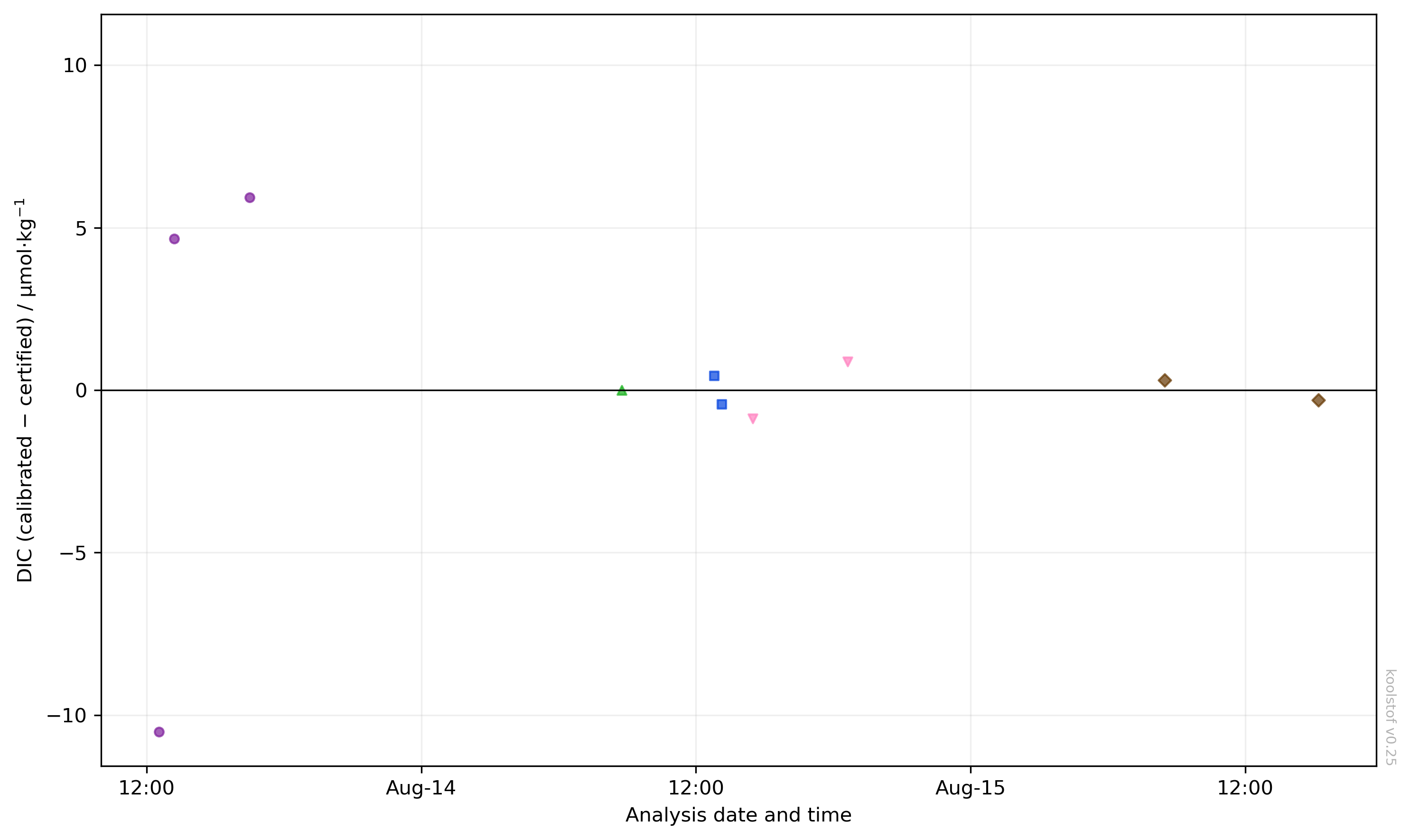
The CRMs for each analysis session will fall on average at zero. The scatter about zero gives some indication of the precision of the measurement.

In this example, we might also consider checking the lab notebook to see if there are any reasons why the lower purple point in the first session could be excluded from the calibration.

Summary

A complete example of your calibration code might look something like this (the first part is copied from the example higher up the page):

import numpy as np
from koolstof import vindta as ksv

# Import files from VINDTA
logfile = ksv.read_logfile("path/to/logfile.bak")
dbs = ksv.read_dbs("path/to/dbsfile.dbs")

# Assign certified DIC for CRMs
# - In this example, we assume that the 'bottle' column of the dbs always
#   starts with the letters "CRM" for CRMs, and that all CRMs have a
#   certified value of 2017.45 µmol/kg
dbs["dic_certified"] = np.where(
    dbs.bottle.str.startswith("CRM"), 2017.45, np.nan
)

# Assign analysis temperature, if it's not 25 °C
dbs["temperature_analysis_dic"] = 23.0

# Assign dbs["salinity"] here too, if it's not always 35

# Set up logicals
dbs["blank_good"] = True
dbs["k_dic_good"] = ~dbs.dic_certified.isnull()

# Here, set any values of dbs.blank_good to False as needed from looking
# at the figures below 

# Find and apply blank corrections
sessions = ksv.blank_correction(dbs, use_from=8)

# Visualise blank corrections
ksv.plot_increments(dbs, logfile)
ksv.plot_blanks(dbs, sessions)

# Here, set any values of dbs.k_dic_good to False as needed from looking
# at the figures below

# Calibrate DIC
ksv.calibrate_dic(dbs, sessions)

# Visualise the calibration
ksv.plot_k_dic(dbs, sessions, show_ignored=False)
ksv.plot_dic_offset(dbs, sessions)